Florian STDP

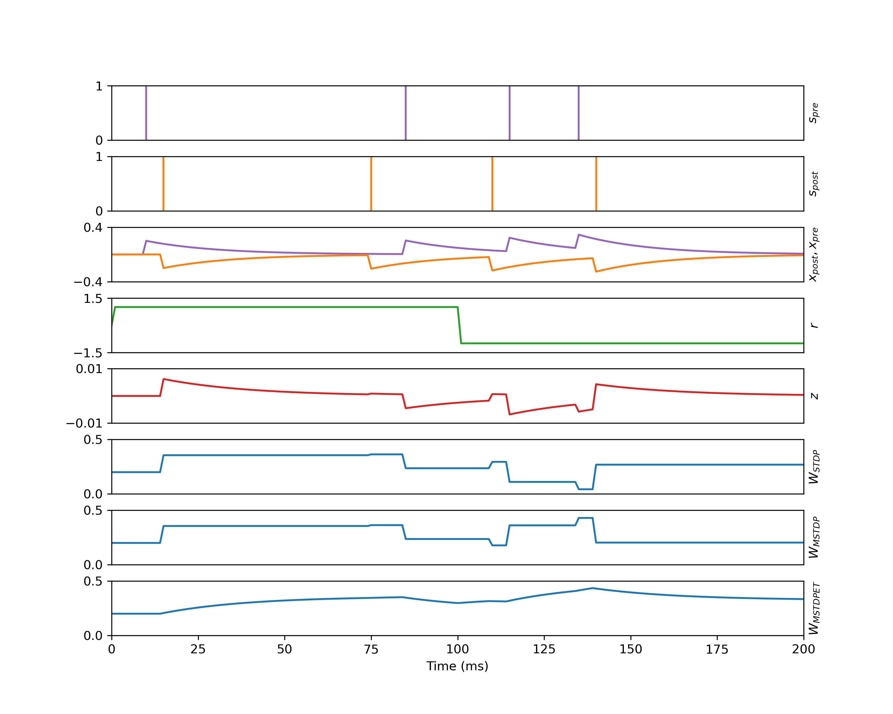
A demonstration replicating a comparison between spike-timing dependent plasticity (STDP), modulated spike-timing dependent plasticity (MSTDP), and modulated spike-timing dependent plasticity with eligibility trace (MSTDPET) given in 10.1162/neco.2007.19.6.1468.

Download this example as a Python script or as a Jupyter notebook .

import inferno
from inferno.extra import ExactNeuron
from inferno.learn import STDP, MSTDP, MSTDPET
from inferno.neural import DeltaCurrent, LinearDirect, Serial
import torch
import matplotlib.pyplot as plt

Set the Training Hyperparameters

Here, lr_post and lr_pre correspond to the amplitude of the spike trace used for calculating the weight update on a postsynaptic spike and presynaptic spike respectively. The time constant for both spike traces is tc_spike and for the eligibility trace is tc_elig. The weight is initialized to w_init and the magnitude of the reward term is reward_mag.

lr_post = 0.2
lr_pre = -0.2
tc_spike = 20.0
tc_elig = 25.0
w_init = 0.2
reward_mag = 1.0

Construct the Layers

For this example, we’re using the ExactNeuron provided by inferno.extra. This lets us specify the desired output in order to compare STDP, MSTDP, and MSTDPET without needing to concern ourselves with the specific neuronal dynamics.

stdp_layer = Serial(
    LinearDirect(
        (1,),
        1.0,
        synapse=DeltaCurrent.partialconstructor(1.0),
        weight_init=lambda x: inferno.full(x, w_init),
    ),
    ExactNeuron((1,), 1.0, rest_v=-60, thresh_v=-40),
)
stdp_layer.connection.updater = stdp_layer.connection.defaultupdater()

mstdp_layer = Serial(
    LinearDirect(
        (1,),
        1.0,
        synapse=DeltaCurrent.partialconstructor(1.0),
        weight_init=lambda x: inferno.full(x, w_init),
    ),
    ExactNeuron((1,), 1.0, rest_v=-60, thresh_v=-40),
)
mstdp_layer.connection.updater = mstdp_layer.connection.defaultupdater()

mstdpet_layer = Serial(
    LinearDirect(
        (1,),
        1.0,
        synapse=DeltaCurrent.partialconstructor(1.0),
        weight_init=lambda x: inferno.full(x, w_init),
    ),
    ExactNeuron((1,), 1.0, rest_v=-60, thresh_v=-40),
)
mstdpet_layer.connection.updater = mstdpet_layer.connection.defaultupdater()

Construct the Trainers

For this demo, we’ll be using the trainers provided by Inferno: STDP, MSTDP, and MSTDPET.

stdp_trainer = STDP(lr_post, lr_pre, tc_spike, tc_spike)
_ = stdp_trainer.register_cell("only", stdp_layer.cell)

mstdp_trainer = MSTDP(lr_post, lr_pre, tc_spike, tc_spike)
_ = mstdp_trainer.register_cell("only", mstdp_layer.cell)

mstdpet_trainer = MSTDPET(lr_post, lr_pre, tc_spike, tc_spike, tc_elig)
_ = mstdpet_trainer.register_cell("only", mstdpet_layer.cell)

Configure Spike and Reward Generation

presyn_times = [10, 85, 115, 135]
postsyn_times = [15, 75, 110, 140]

def spikes(step: int) -> tuple[torch.Tensor, torch.Tensor]:
    if step in presyn_times:
        pre = torch.ones((1, 1), dtype=torch.bool)
    else:
        pre = torch.zeros((1, 1), dtype=torch.bool)

    if step in postsyn_times:
        post = torch.ones((1, 1), dtype=torch.bool)
    else:
        post = torch.zeros((1, 1), dtype=torch.bool)

    return pre, post

def rewardfn(step: int) -> float:
    if step <= 100:
        return reward_mag
    else:
        return -reward_mag

Log and Perform the Updates

time = torch.arange(0, 201, 1, dtype=torch.float32)

w_stdp = torch.zeros_like(time)
w_stdp[0] = w_init
w_mstdp = torch.zeros_like(time)
w_mstdp[0] = w_init
w_mstdpet = torch.zeros_like(time)
w_mstdpet[0] = w_init

presyn_spikes = torch.tensor(presyn_times, dtype=torch.float32)
postsyn_spikes = torch.tensor(postsyn_times, dtype=torch.float32)
presyn_trace = torch.zeros_like(time)
postsyn_trace = torch.zeros_like(time)

elig_trace = torch.zeros_like(time)

reward = torch.zeros_like(time)

for step in range(1, 201):
    # determine pre/post spikes and reward
    pre, post = spikes(step)
    r = rewardfn(step)

    # process inputs
    _ = stdp_layer(pre, neuron_kwargs={"override": post})
    _ = mstdp_layer(pre, neuron_kwargs={"override": post})
    _ = mstdpet_layer(pre, neuron_kwargs={"override": post})

    # apply updates
    stdp_trainer()
    stdp_layer.connection.update()
    mstdp_trainer(r)
    mstdp_layer.connection.update()
    mstdpet_trainer(r)
    mstdpet_layer.connection.update()

    # record state
    w_stdp[step] = stdp_layer.connection.weight.item()
    w_mstdp[step] = mstdp_layer.connection.weight.item()
    w_mstdpet[step] = mstdpet_layer.connection.weight.item()

    presyn_trace[step] = mstdp_trainer.get_monitor("only", "trace_pre").peek().item()
    postsyn_trace[step] = -mstdp_trainer.get_monitor("only", "trace_post").peek().item()

    elig_trace[step] = (
        mstdpet_trainer.get_monitor("only", "elig_post").peek().item()
        - mstdpet_trainer.get_monitor("only", "elig_pre").peek().item()
    )

    reward[step] = r

Plot the Results

Note that if precisely trying to replicate the results from 10.1162/neco.2007.19.6.1468, there may be some difficult as the potentiative and depressive learning rates are incorporated directly into the calculation of eligibility. In order to achieve the exact results described, the postsynaptic and presynaptic learning rates should be set to 1.0 and -1.0 respectively, then the scale parameter should be set to the magnitude of the desired learning rate.

fig, axs = plt.subplots(nrows=8, ncols=1, sharex=True, figsize=(10, 8))

axs[0].set_xlim(0, 200)
for ax in axs[:-1]:
    plt.setp(ax.get_xticklabels(), visible=False)
    ax.tick_params(axis='x', which='both', bottom=False)
    ax.yaxis.set_label_position("right")
axs[-1].yaxis.set_label_position("right")

# presyn spikes
axs[0].vlines(presyn_spikes.numpy(), 0.0, 1.0, colors="tab:purple")
axs[0].set_ylim(0.0, 1.0)
axs[0].set_yticks([0.0, 1.0])
axs[0].set_ylabel(r"$s_{pre}$")

# postsyn spikes
axs[1].vlines(postsyn_spikes.numpy(), 0.0, 1.0, colors="tab:orange")
axs[1].set_ylim(0.0, 1.0)
axs[1].set_yticks([0.0, 1.0])
axs[1].set_ylabel(r"$s_{post}$")

# spike trace
axs[2].plot(time.numpy(), presyn_trace.numpy(), c="tab:purple")
axs[2].plot(time.numpy(), postsyn_trace.numpy(), c="tab:orange")
axs[2].set_ylim(-0.4, 0.4)
axs[2].set_yticks([-0.4, 0.4])
axs[2].set_ylabel(r"$x_{post}, x_{pre}$")

# reward
axs[3].plot(time.numpy(), reward.numpy(), c="tab:green")
axs[3].set_ylim(-1.5, 1.5)
axs[3].set_yticks([-1.5, 1.5])
axs[3].set_ylabel(r"$r$")

# eligibility trace
axs[4].plot(time.numpy(), elig_trace.numpy(), c="tab:red")
axs[4].set_ylim(-1e-2, 1e-2)
axs[4].set_yticks([-1e-2, 1e-2])
axs[4].set_ylabel(r"$z$")

# weights (updated with STDP)
axs[5].plot(time.numpy(), w_stdp.numpy(), c="tab:blue")
axs[5].set_ylim(0.0, 0.5)
axs[5].set_yticks([0.0, 0.5])
axs[5].set_ylabel(r"$W_{STDP}$")

# weights (updated with MSTDP)
axs[6].plot(time.numpy(), w_mstdp.numpy(), c="tab:blue")
axs[6].set_ylim(0.0, 0.5)
axs[6].set_yticks([0.0, 0.5])
axs[6].set_ylabel(r"$W_{MSTDP}$")

# weights (updated with MSTDPET)
axs[7].plot(time.numpy(), w_mstdpet.numpy(), c="tab:blue")
axs[7].set_ylim(0.0, 0.5)
axs[7].set_yticks([0.0, 0.5])
axs[7].set_ylabel(r"$W_{MSTDPET}$")
axs[7].set_xlabel(r"Time (ms)")

plt.subplots_adjust(hspace=0.3)
plt.show()